How to Calculate Compound Interest in Excel

How to Calculate Compound Interest in Excel

Being able to accurately calculate compound interest is a great way to forecast how an investment or your savings grow over time. But instead of doing this calculation manually for every investment or forecast, did you know you can build a compound interest calculator in Excel that does the work for you?

While building this might seem daunting, it’s actually a relatively simple process. This guide offers you clear step-by-step instructions for how to build the calculator in minutes, even if you’re not an expert in Excel.

Step-by-Step Guide for Calculating Compound Interest in Excel

Here’s a closer look at the steps involved in creating a compound interest calculator in Excel.

1. Set Your Inputs

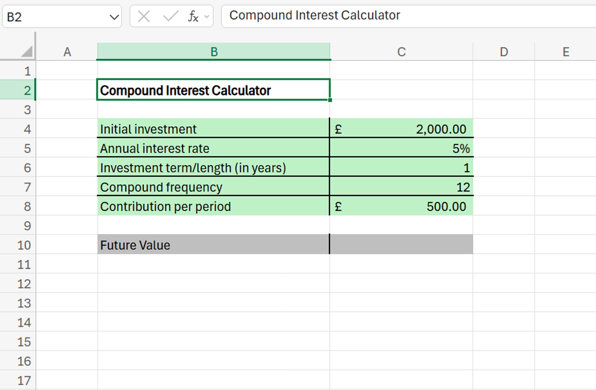
The first step is to add all of the required inputs and set them to the proper amounts. The inputs you need to include are:

• Initial investment: The amount you’re starting with.
• Annual interest rate: The percentage earned by your investment or savings in a year.
• The investment term/length: How long you’ll be saving or investing for.
• Compound frequency: How often the interest compounds.
• Contribution per period: How much you contribute per period.

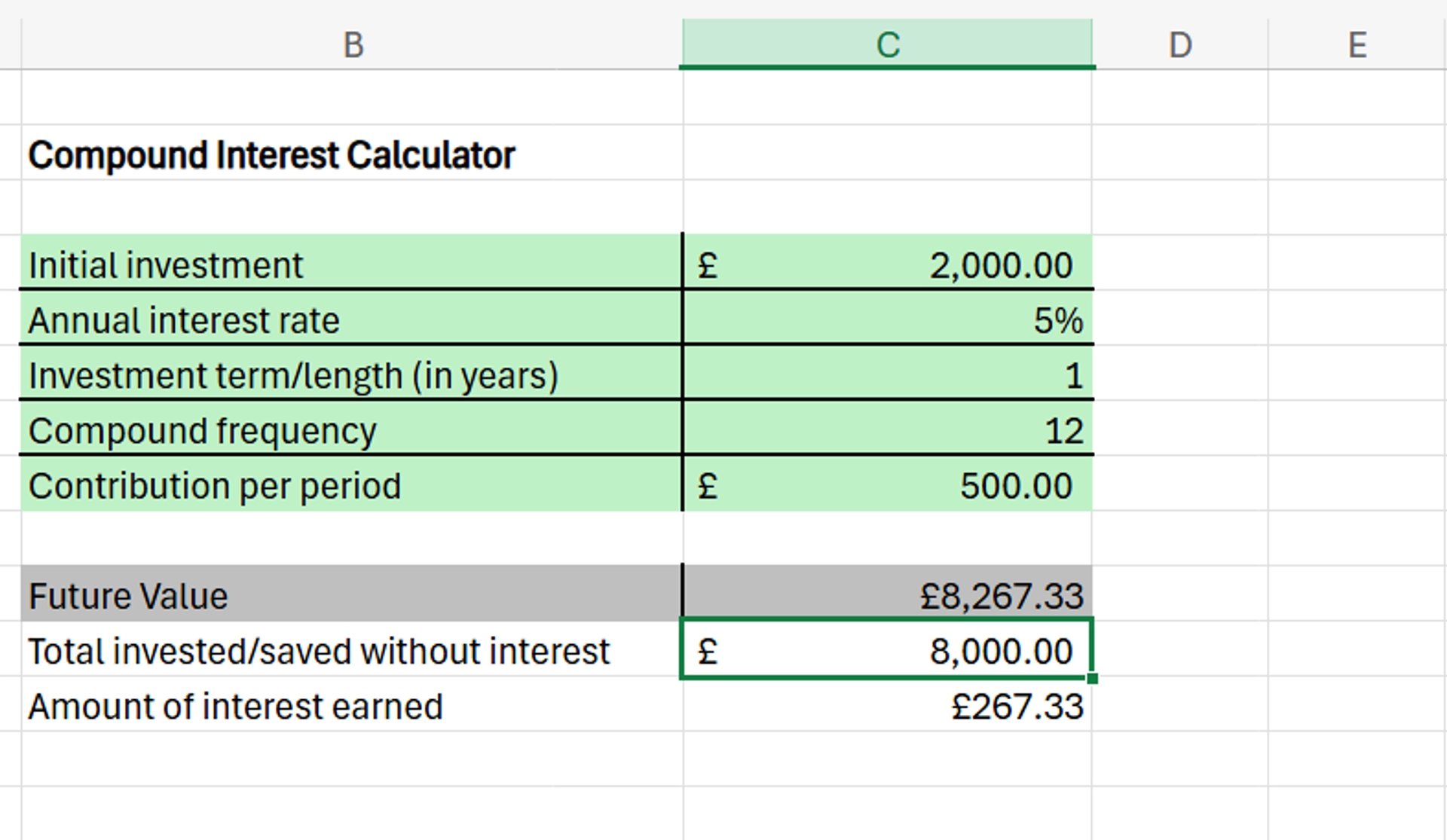
For this example, we’re using an initial investment of £2,000, an annual interest rate of 5%, an investment length of 1 year, with monthly compounding (12 compound periods), and a £500 contribution per period.

Also, under the calculator, add a “Future Value” line, which is where you’ll be able to see the future value of your investment/savings.

2. Use the Future Value (FV) Function and The Compound Interest in Excel Formula

Once you have the proper inputs and numbers/percentages in place, it’s time to use the Future Value (FV) function to calculate the compound interest in Excel. To begin, type =FV in the cell next to “Future Value” and select the FV function.

First, you’ll enter the rate, but due to it being an annual rate, you’ll need to divide the annual rate by the compound frequency. In our example, this means 5 divided by 12.

Next, enter the number of compounding periods, which is the investment term/length multiplied by the compound frequency. Again, in our example, this means 1 times 12.

After that, add the contribution per period, as well as the initial investment. At the end of the calculation, add a 1 to signify that the payment takes place at the start of each period, not the end.

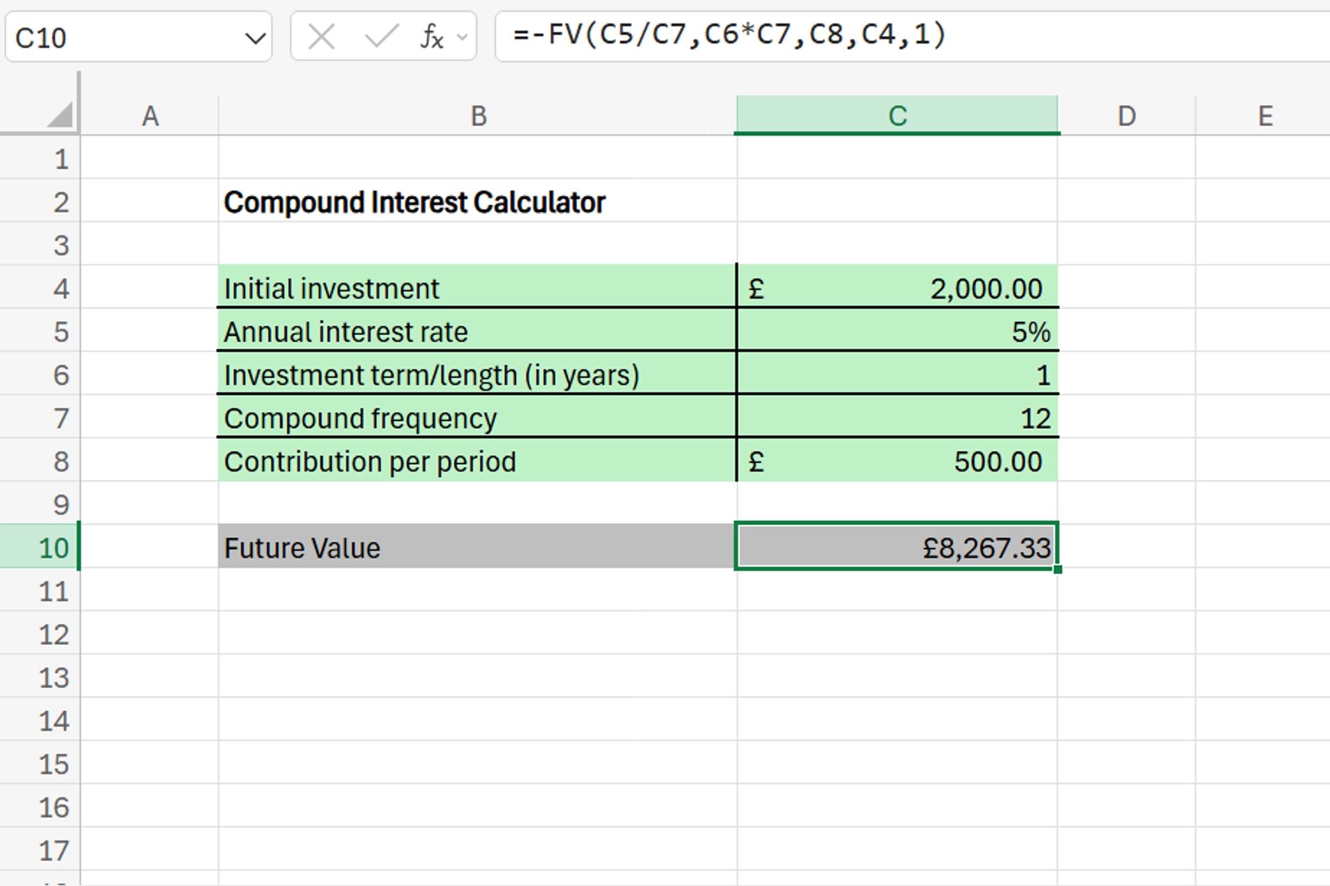
Once this is done, you’ll see that the compound interest formula in Excel​ is: =FV(rate/cfreq,term*cfreq,cper,ii,1)

This formula uses these meanings:

• rate - annual rate
• cfreq - compound frequency
• term - investment term/length
• cper - contribution per period
• ii - initial investment

Don’t forget to separate the inputs by a comma to ensure the calculator works properly.

Before clicking enter and seeing your results, make sure to add a negative sign in front of the formula, to ensure the results are positive.

After completing all of these steps in our example, we’re able to see here that the future value of our investment is £8,267.33.

3. Verify With a Calculation Table

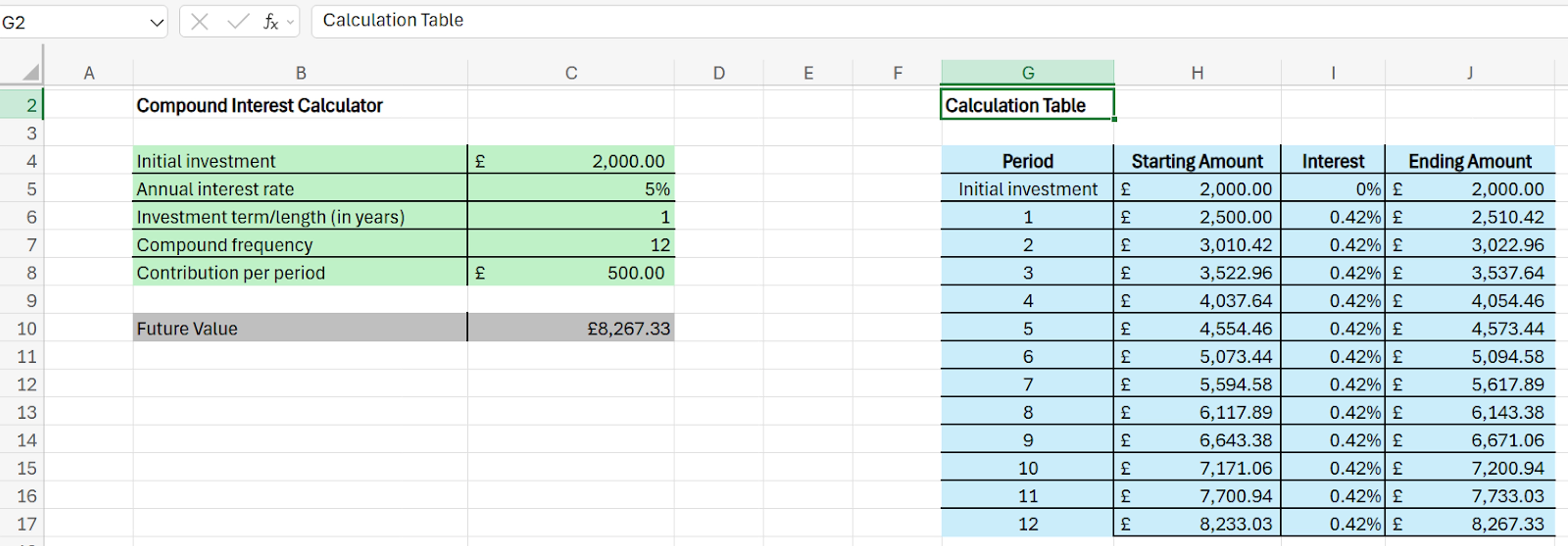
The final step in the process is to verify that the calculator is working properly to ensure you end up with correct results. We can do this by building a calculation table next to the calculator.

To do this, create four columns titled Period, Starting Amount, Interest, and Ending Amount. Each column should be 13 cells long. In the “Period” column, the first cell should contain “Initial investment”, and the rest should include the numbers 1 through 12, to represent each month/compound frequency.

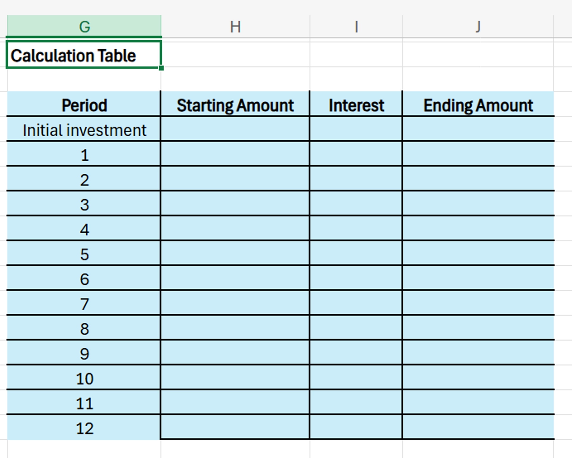
For each of these 13 rows, we’re going to calculate the amount at the start of each month, the interest earned for that month, and the amount at the end of the month.

Begin in the “Starting Amount” column right next to “Initial Invesment”, and add an equal sign (=) followed by your initial investment amount. In the “Interest” column, input 0% as there hasn’t been any interest earned yet.

In the “Ending Amount” column, add the following formula: =startii*(1+mint).

This formula and the next use the same meanings as the previous formula, plus:

• startii - the amount in the Starting Amount column in the Initial Investment row
• start - the amount in the Starting Amount Column in the Month 1 row
• end - The amount in the Ending Amount column
• mint - monthly interest (the amount in the Interest column)

Moving onto the “Starting Amount” column for month 1, add the following formula: =end+cper. But before hitting enter, add absolute references to the “Contributions per period” value, to ensure it remains static and doesn’t change from cell to cell, which dramatically speeds up the process and stops you from having to manually add it each time.

Doing this is easy, as all you need to do is add a $ sign before the row and column in the value.

Moving over to the “Interest Column” in month 1, add the formula: =rate/cfreq, but before hitting enter, add absolute references to both of these values to keep them static.

Finally, moving over to the “Ending Amount” column for month 1, add this formula: =start*(1+mint). Once that’s done, simply select the month 1 row and double click the bottom right-hand corner of the “Ending Amount” column. This will automatically bring all of these formulas down to the rest of the table and complete the calculations automatically.

If the amount in the “Ending Amount” column in month 12 is the same as the “Future Value” line under the calculator, you can see that it works properly. Of course, you can also change the input figures and amounts to test the model even further.

4. Checking the Interest Earned

While the tool now works and you can easily use it to calculate compound interest in Excel, what if you want to just specifically see the amount of interest earned? To do this, go back to the compound interest calculator and calculate the amount saved/invested without interest, and subtract it from the total future value.

The formula for calculating the amount saved without interest is: =ii+cper*term*cfreq.

From there, simply subtract this number from the Future Value to end up with the amount of interest you earned.

In our example, the formula is =2,000+500*1*12, which equals 8,000. After subtracting 8,000 from 8,267.33, we can see that £267.33 of interest was earned.

Potential Business Applications for Calculating Compound Interest in Excel

Being able to calculate compound interest in Excel is incredibly useful for planning investments, forecasting, and even analysing financial performance. It’ll save you and your organisation plenty of time compared to handling the calculations manually.

The techniques you use to create this compound interest calculator can also be used to help build dynamic and complex charts and financial models to streamline and simplify your decision-making in the future, as well.

Check out our dedicated article for a detailed guide to ensure you can fully grasp the concept of calculating compound interest in Excel.

FAQs

Here are a few frequently asked questions about how to calculate compound interest in Excel, along with their answers.

How do I calculate compound interest in Excel?

To calculate compound interest in Excel, you need to begin by setting your inputs, using the FV function properly, and creating a calculation table to verify that everything is working correctly.

What is the formula for compound interest in Excel?

The compound interest formula in Excel is: =FV(rate/cfreq,term*cfreq,cper,ii,1). In this formula, “rate” is the annual interest rate, “cfreq” is compound frequency, “term” is the investment term/length, “cper” is contribution per period, and “ii” is the initial investment.