How to Password Protect Excel & Hide a Single Column

How to Password Protect Excel and Hide Just One Column in a Master Spreadsheet

You can never be too careful when working with several people on a spreadsheet. You may need to hide sensitive data and lock the document.

Follow our step-by-step guide to hide columns and password-protect an Excel worksheet.

Unlock All Cells

Unlocking all the cells in the sheet ensures that only the specific columns or cells you select are locked when you protect the sheet.

Tip: By default, all the cells in Excel are locked but this only takes effect when you protect the sheet.

1. Navigate to the Select All button and select it. The button is found at the top-left corner of the sheet where the row numbers and column letters intersect.

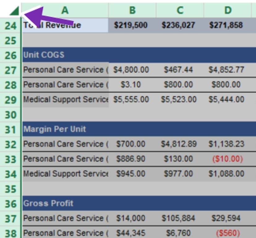
2. Right-click any cell or area in the sheet.

3. Select Format Cells from the menu.

4. In the dialog box, select Protection

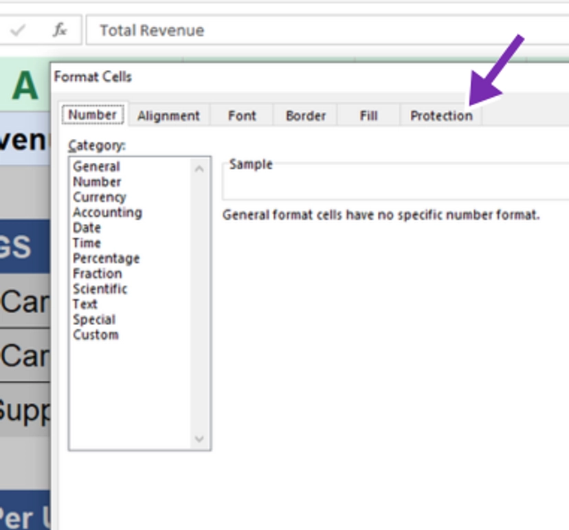
5. Uncheck Locked and select OK.

Lock the Columns You Want to Protect

Columns are represented by letters while numbers represent rows.

1. Select the letter that represents the column you want to lock.

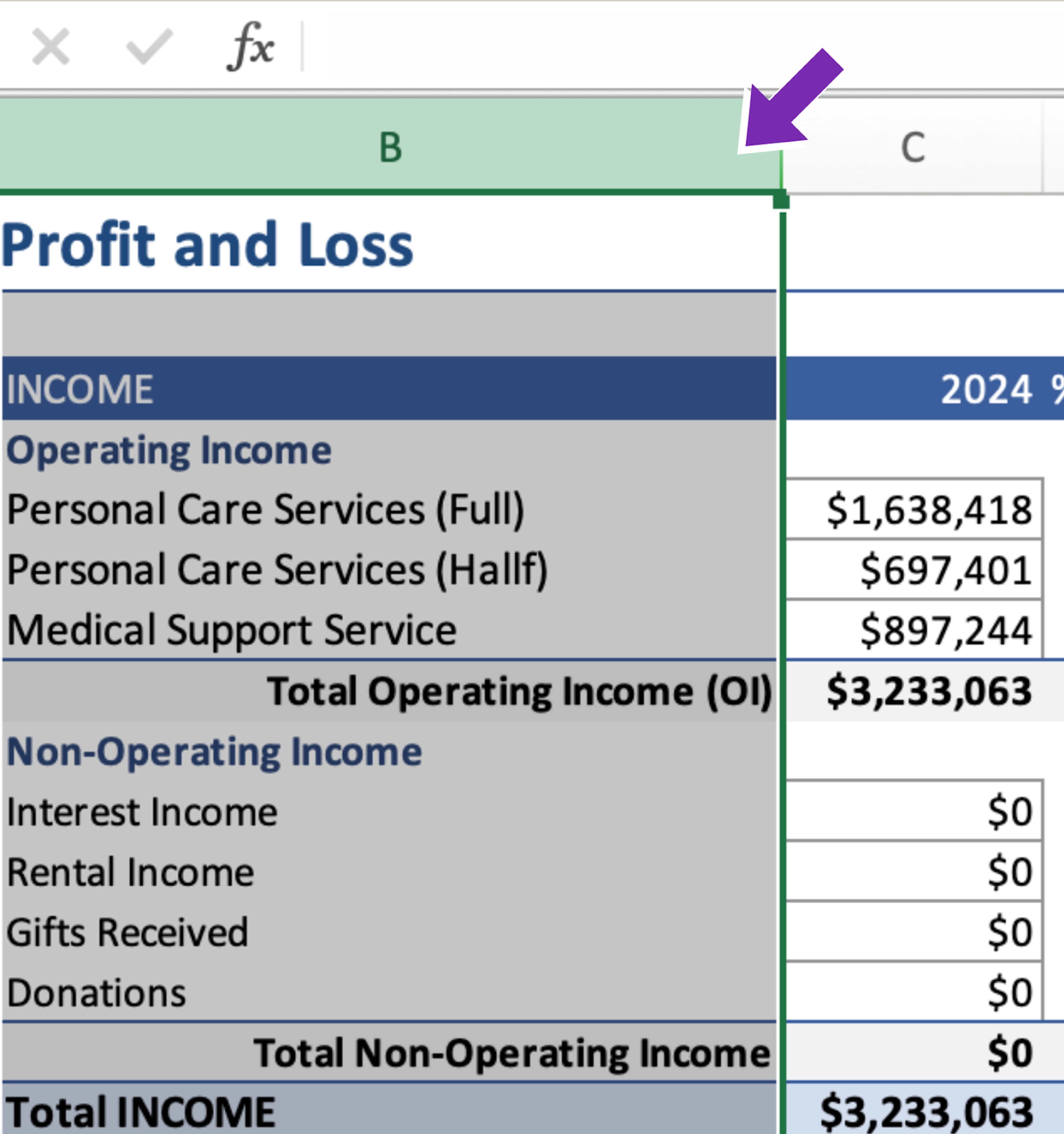
2. Right-click the selected column.

3. Select Format Cells from the menu.

4. Select Protection in the dialog box.

5. Check the Locked option and select OK.

6. To hide the locked column, right-click anywhere on the selected column and choose Hide.

Protect the Sheet

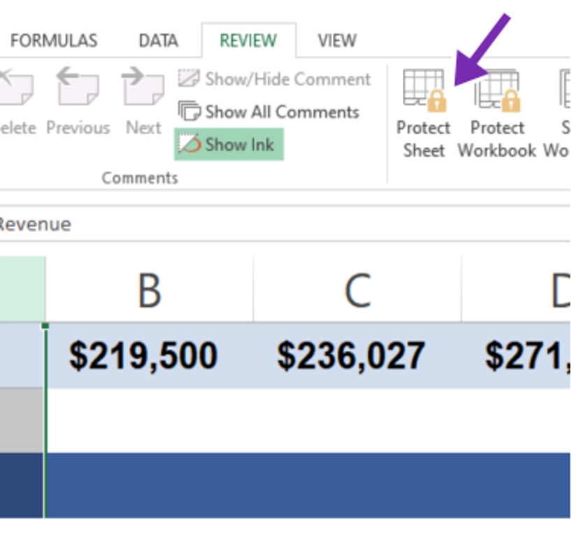
1. Navigate to the Review tab on the Ribbon and select it. The Ribbon, also known as the toolbar, is at the top of the Excel window. The ribbon houses several tabs, including File, Home, Review, Data, and Formulas.

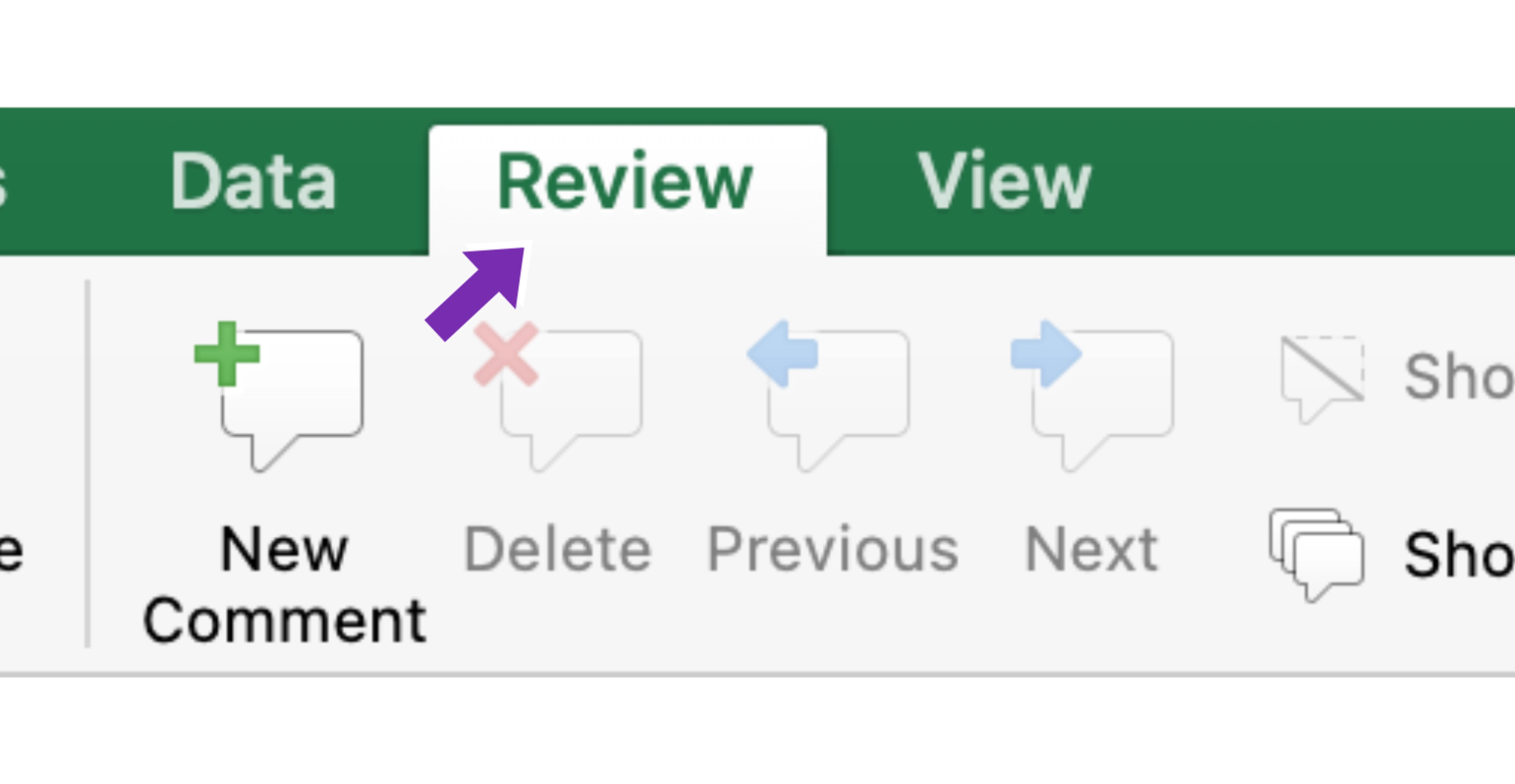
2. Select Protect Sheet.

3. In the dialog box, enter a password to password-protect your worksheet. You can also set user permission or role by checking and unchecking necessary boxes.

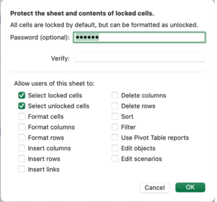
4. Re-enter your password and select OK.

You can still access the rest of the unlocked rows and columns but must provide a password to access the locked columns.

Can People Still Access Excel Worksheet after Protecting It with a Password?

Protecting your worksheet with a password should block unauthorised access. However, even without a password, some people may use third-party apps to gain entry. Use the Backstage View in the File tab for advanced security.